Comparing within and between Gene Sets

Within sets selected by a single tool this problem is often addressed by said tool. For between and combined sets a ranking method or measure is less obvious. Here we demonstrate the use of random forest feature importances and derived scores with those from the DGE demonstrated in the tour notebook to score genes.

# OS-independent path management.
from os import  environ
from pathlib import Path
import numpy as np
import pandas as pd
import holoviews as hv
from sklearn import model_selection
from sklearn.ensemble import RandomForestClassifier
import umap
import umap.plot
import GSForge as gsf
import matplotlib.pyplot as plt
import seaborn as sns
hv.extension("bokeh")

OSF_PATH = Path(environ.get("GSFORGE_DEMO_DATA", default="~/GSForge_demo_data/")).expanduser().joinpath("osfstorage", "oryza_sativa")
NORMED_GEM_PATH = OSF_PATH.joinpath("AnnotatedGEMs", "oryza_sativa_hisat2_normed.nc")
LIT_DGE_GSC_PATH = OSF_PATH.joinpath("GeneSetCollections", "literature", "DGE")
LIT_TF_PATH = OSF_PATH.joinpath("GeneSetCollections", "literature", "TF")
TOUR_BORUTA = OSF_PATH.joinpath("GeneSetCollections", "tour_boruta")
TOUR_DGE = OSF_PATH.joinpath("GeneSetCollections", "DEG_gene_sets")

agem = gsf.AnnotatedGEM(NORMED_GEM_PATH)

%%time
lit_dge_coll = gsf.GeneSetCollection.from_folder(gem=agem, target_dir=LIT_DGE_GSC_PATH, name="Literature DGE")
lit_tf_coll = gsf.GeneSetCollection.from_folder(gem=agem, target_dir=LIT_TF_PATH, name="Literature TF")
boruta_gsc = gsf.GeneSetCollection.from_folder(gem=agem, target_dir=TOUR_BORUTA, name="Boruta Results")
tf_geneset = gsf.GeneSet.from_GeneSets(*list(lit_tf_coll.gene_sets.values()), name='transcription factors')
tour_dge_coll = gsf.GeneSetCollection.from_folder(gem=agem, target_dir=TOUR_DGE, name="Tour DGE")

CPU times: user 25.6 s, sys: 224 ms, total: 25.9 s
Wall time: 25.9 s

combined_gsc = gsf.GeneSetCollection(
    gem=agem,                          
    gene_sets={**boruta_gsc.gene_sets, 
               **lit_dge_coll.gene_sets, 
               **tour_dge_coll.gene_sets, 
               'transcription factors': tf_geneset})

combined_gsc.summarize_gene_sets()

{'edgeR filter': 21915,
 "'0 + treatment:genotype'__treatment[HEAT]": 4071,
 "'0 + treatment:genotype'__treatment[RECOV_HEAT]": 3719,
 "'0 + treatment:genotype'__treatment[DROUGHT]": 3703,
 "'0 + treatment:genotype'__treatment[RECOV_DROUGHT]": 2806,
 'DROUGHT_UP': 1175,
 'Boruta_treatment': 771,
 'Boruta_genotype': 663,
 'HEAT_UP': 592,
 'RECOV_DROUGHT_UP': 446,
 "'0 + treatment'__treatment[DROUGHT]": 359,
 'transcription factors': 276,
 "'0 + treatment'__treatment[HEAT]": 222,
 "'0 + treatment'__treatment[RECOV_DROUGHT]": 181,
 'DROUGHT_DOWN': 170,
 'HEAT_DOWN': 106,
 "'0 + treatment'__treatment[RECOV_HEAT]": 99,
 'RECOV_HEAT_UP': 76,
 'RECOV_DROUGHT_DOWN': 58,
 'RECOV_HEAT_DOWN': 43}

Rank Genes with a Random Forest

Random forests and feature ranks. Robust enough to function in our case. Some values filtered prior to dge analysis…

gene_rank_mdl = RandomForestClassifier(
    class_weight='balanced', 
    n_estimators=1000, 
    n_jobs=-2,
    max_depth=5,
    min_samples_split=2,
    min_samples_leaf=1,
    min_weight_fraction_leaf=0.0,
    max_features='auto',
)

treatment_feature_importance = gsf.operations.RankGenesByModel(
    combined_gsc,
    selected_gene_sets=["Boruta_treatment", "'0 + treatment:genotype'__treatment[HEAT]"],
    gene_set_mode="union",
    annotation_variables=["treatment"],
    model=gene_rank_mdl,
    n_iterations=5
)

treatment_nFDR = gsf.operations.nFDR(
    combined_gsc,
    selected_gene_sets=["Boruta_treatment", "'0 + treatment:genotype'__treatment[HEAT]"],
    gene_set_mode="union",
    annotation_variables=["treatment"],
    model=gene_rank_mdl,
    n_iterations=5
)

dge_ds = tour_dge_coll["'0 + treatment:genotype'__treatment[HEAT]"]
gene_union = combined_gsc.union(["Boruta_treatment", "'0 + treatment:genotype'__treatment[HEAT]"])
boruta_support = np.isin(gene_union, combined_gsc["Boruta_treatment"].get_support())
dge_support = np.isin(gene_union, dge_ds.get_support())

support_source = np.zeros_like(gene_union)
support_source[boruta_support] = "Boruta"
support_source[dge_support] = "DGE"
support_source[(boruta_support * dge_support) == True] = "Both"


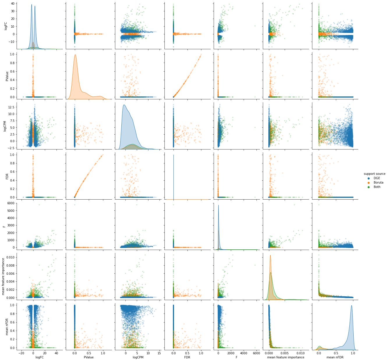
df = pd.DataFrame({
    "logFC": dge_ds.data['logFC'].reindex(Gene=gene_union).values,
    "PValue": dge_ds.data['PValue'].reindex(Gene=gene_union).values,
    "logCPM": dge_ds.data['logCPM'].reindex(Gene=gene_union).values,
    "FDR": dge_ds.data['FDR'].reindex(Gene=gene_union).values,
    "F": dge_ds.data['F'].reindex(Gene=gene_union).values,
    "Gene": gene_union,
    "mean feature importance": treatment_feature_importance.mean(dim='model_iteration').values,
    "mean nFDR": treatment_nFDR.mean(dim='model_iteration').values,
    "support source": support_source,
}).set_index("Gene")

sns.pairplot(df, hue="support source", markers='.', diag_kind="kde", 
             plot_kws=dict(edgecolor=None, alpha=0.25));

/home/tyler/anaconda3/envs/gsfenv/lib/python3.7/site-packages/seaborn/distributions.py:305: UserWarning: Dataset has 0 variance; skipping density estimate.
  warnings.warn(msg, UserWarning)
/home/tyler/anaconda3/envs/gsfenv/lib/python3.7/site-packages/seaborn/distributions.py:305: UserWarning: Dataset has 0 variance; skipping density estimate.
  warnings.warn(msg, UserWarning)
/home/tyler/anaconda3/envs/gsfenv/lib/python3.7/site-packages/seaborn/distributions.py:305: UserWarning: Dataset has 0 variance; skipping density estimate.
  warnings.warn(msg, UserWarning)

<seaborn.axisgrid.PairGrid at 0x7f5595006ad0>

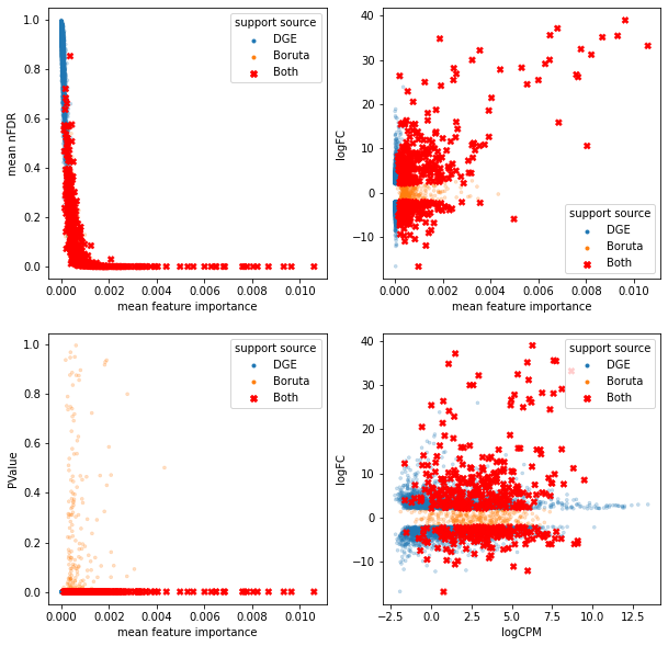
bdf = df[support_source == "Both"]
sdf = df[~(support_source == "Both")]

fig, axes = plt.subplots(2, 2, figsize=(10, 10))
axes = axes.flatten()

sns.scatterplot(data=sdf, x='mean feature importance', y='mean nFDR', hue='support source',
                edgecolor=None, alpha=0.25, markers=['.', '.'], 
                style='support source', ax=axes[0]);
sns.scatterplot(data=sdf, x='mean feature importance', y='logFC', hue='support source',
                edgecolor=None, alpha=0.25, markers=['.', '.'], 
                style='support source', ax=axes[1]);
sns.scatterplot(data=sdf, x='mean feature importance', y='PValue', hue='support source',
                edgecolor=None, alpha=0.25, markers=['.', '.'], 
                style='support source', ax=axes[2]);
sns.scatterplot(data=sdf, x='logCPM', y='logFC', hue='support source',
                edgecolor=None, alpha=0.25, markers=['.', '.'], 
                style='support source', ax=axes[3]);

sns.scatterplot(data=bdf, x='mean feature importance', y='mean nFDR', hue='support source',
                edgecolor=None, alpha=1, markers=['X'], palette=['red'],
                style='support source', ax=axes[0]);
sns.scatterplot(data=bdf, x='mean feature importance', y='logFC', hue='support source',
                edgecolor=None, alpha=1, markers=['X'], palette=['red'],
                style='support source', ax=axes[1]);
sns.scatterplot(data=bdf, x='mean feature importance', y='PValue', hue='support source',
                edgecolor=None, alpha=1, markers=['X'], palette=['red'],
                style='support source', ax=axes[2]);
sns.scatterplot(data=bdf, x='logCPM', y='logFC', hue='support source',
                edgecolor=None, alpha=1, markers=['X'], palette=['red'],
                style='support source', ax=axes[3]);

<AxesSubplot:xlabel='logCPM', ylabel='logFC'>

Compare Gene Selections using Machine-Learning Models

We can estimate how well a given subset of genes ‘describes’ a sample (phenotype) label by comparing how well they perform using a given machine learning model.

In the example below, a simple random forest is demonstrated.

from sklearn.linear_model import Perceptron, RidgeClassifier

collections = list(combined_gsc.gene_sets.keys())
results = {}

for collection in collections:
#     print(collection)
    counts, treatment = gsf.get_gem_data(combined_gsc, selected_gene_sets=[collection], annotation_variables="treatment")
    
    x_train, x_test, y_train, y_test = model_selection.train_test_split(counts.values, treatment.values, random_state=42)
    
    model_a = Perceptron(random_state=42).fit(x_train, y_train)
    model_b = RidgeClassifier(random_state=42).fit(x_train, y_train)
    model_c = RandomForestClassifier(random_state=42).fit(x_train, y_train)

    results[(collection, 'Perceptron')] = model_a.score(x_test, y_test)
    results[(collection, 'RidgeClassifier')] = model_b.score(x_test, y_test)
    results[(collection, 'RandomForestClassifier')] = model_c.score(x_test, y_test)    

hv.Bars(results, ["Model", "Gene Selection Group"], "Score").opts(
    xrotation=90, invert_axes=True, width=800, ylim=(0, 1.1), height=600, multi_level=False)

This does not necessarily mean that one set is more complete, or better than another. Keep in mind:

• A similar model was used to ‘select’ the features as was used to ‘test’.

• This has nothing (directly) to do with biology.

• Model scores may not be stable.

With the above (and more) considerations in mind:

• A ‘good’ selection should preform better than using the entire dataset.

• Our selection should be better than guessing, or a random gene set of similar size.

results = pd.Series(results)
results[results > results.quantile(.9)]
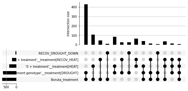
top_results = results[results > results.quantile(.9)].index.get_level_values(0).values
top_results
# top_results.index.levels[0]

array(['Boruta_treatment', 'Boruta_treatment', 'RECOV_DROUGHT_DOWN',
       "'0 + treatment:genotype'__treatment[DROUGHT]",
       "'0 + treatment'__treatment[RECOV_HEAT]",
       "'0 + treatment'__treatment[HEAT]"], dtype=object)

gsf.plots.collections.UpsetPlotInterface(combined_gsc, selected_gene_sets=top_results)

<upsetplot.plotting.UpSet at 0x7f55941d6ed0>

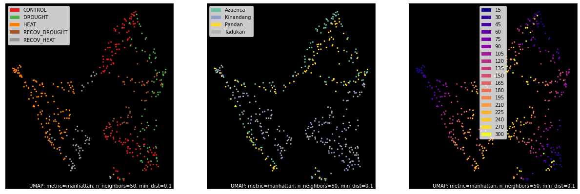
counts, labels = gsf.get_gem_data(combined_gsc, 
                                  selected_gene_sets=top_results.tolist(),
                                  annotation_variables=['treatment', 'genotype', 'time'], 
                                  count_variable='tmm_counts',
                                 )
mapper = umap.UMAP(random_state=42, metric='manhattan', densmap=False, n_neighbors=50).fit(counts.values)

fig, axes = plt.subplots(1, 3, figsize=(21, 7))
umap.plot.points(mapper, labels=labels['treatment'], background='black', ax=axes[0], color_key_cmap='Set1');
umap.plot.points(mapper, labels=labels['genotype'], background='black', ax=axes[1], color_key_cmap='Set2');
umap.plot.points(mapper, labels=labels['time'], background='black', ax=axes[2], color_key_cmap='plasma');

<AxesSubplot:>

# treatment_cmap = {
#     'CONTROL': '#1f78b4',
#     'HEAT': '#e31a1c',
#     'RECOV_HEAT': '#fb9a99',
#     'DROUGHT': '#6a3d9a',
#     'RECOV_DROUGHT': '#cab2d6',
# }
# # treatment_cmap

# times = labels['time'].to_series().unique()
# time_colors = hv.plotting.util.process_cmap('viridis', ncolors=len(times), categorical=False)
# time_cmap = {g: c for g, c in zip(times, time_colors)}

# genotypes = labels['genotype'].to_series().unique()
# genotype_colors = hv.plotting.util.process_cmap('set1', ncolors=len(genotypes), categorical=True)
# genotype_cmap = {g: c for g, c in zip(genotypes, genotype_colors)}

# plt.rcParams.update({'font.size': 10, 'font.family': 'serif'})

# fig_inches = 3.5
# fig_dpi = 300
# fig_pixels = int(fig_inches * fig_dpi)

# fig, axes = plt.subplots(figsize=(fig_inches, fig_inches), dpi=fig_dpi)

# colors = labels['treatment'].to_series().map(treatment_cmap).values
# # colors = labels['time'].to_series().map(time_cmap).values
# # colors = labels['genotype'].to_series().map(genotype_cmap).values

# axes.scatter(mapper.embedding_[:, 0], mapper.embedding_[:, 1], s=10, marker='.', linewidths=0, c=colors);


# axes.xaxis.set_visible(False)
# axes.yaxis.set_visible(False)

# for spine in axes.spines.values():
#     spine.set_edgecolor('grey')
#     spine.set_linewidth(0.5)